Introduction
Our goal for this project was to run and tune our Romi robot so that it could follow a course provided by our instructor. To achieve autonomous navigation, we used many sensor systems, starting with quadrature encoders that provided motor feedback for control through PD control. Reflectance sensors enabled us to detect lines on the track surface, allowing for line-following. The IMU supplied orientation data for state estimation and heading correction. A Bluetooth module allowed for wireless data transfer, helpful for running tests. Finally, Bump sensors provided collision detection for obstacle detection.
This Documentation includes information about:
- Hardware
- Software architecture
- Namespaces
- Classes
- Task information
- Test results and performance
- Key takeaways
Authors
- Erik Heuchert
- Alex Power
- Lucas Heuchert
Software architecture
The software architecture can be found by going to the Namespaces, Classes, and Files tabs. There you can find infomation about the files for this project and the functions they contain.
Hardware
Motors
We used Romi, which has two H-bridge motor drivers.
| Purpose | Pin Selection | Function |
|---|---|---|
| Motor Enable Left | PA10 | GPIO |
| Motor Direction Left | PB10 | GPIO |
| Motor Effort Left | PB6 | TIM4_CH1 |
| Motor Enable Right | PC14 | GPIO |
| Motor Direction Right | PC13 | GPIO |
| Motor Effort Right | PB7 | TIM4_CH2 |
Encoders
We used Romi, which has two encoders for their respective motors, allowing us to perform motor control.
| Purpose | Pin Selection | Function |
|---|---|---|
| Encoder Left 1 | PA0 | TIM2_CH1 |
| Encoder Left 2 | PA1 | TIM2_CH2 |
| Encoder Right 1 | PC6 | TIM3_CH1 |
| Encoder Right 2 | PC7 | TIM3_CH2 |
Bluetooth
We used a bluetooth module to send user instructions, as well as receive data for various tests, including step response tests. We attached this to the top of our Romi robit.
| Purpose | Pin Selection | Function |
|---|---|---|
| 5v | E5v | - |
| GND | GND | - |
| UART Tx | C12 | UART5_TX |
| UART Rx | D12 | UART5_RX |
IMU
We used a adafruit bno055, which we configured to IMU mode. This allowed us to things like yaw, pitch, roll and angular velocity. We attached this to the bottom of the Romi robot.
| Purpose | Pin Selection | Function |
|---|---|---|
| IMU | PB9 | SDA |
| IMU | PB8 | SCL |
| IMU REST | PC8 | REST |
Line Sensors
We used a 13 channel reflectance sensor array, with analog output. This allows us to read a line, which we can then use make our Romi robot follow a line. We attached this using 3D printed supports to the front of the robot.
| Purpose | Pin Selection | Function |
|---|---|---|
| Analog Pin 1 | PA6 | Analog |
| Analog Pin 2 | PA7 | Analog |
| Analog Pin 3 | PC4 | Analog |
| Analog Pin 4 | PA0 | Analog |
| Analog Pin 5 | PA1 | Analog |
| Analog Pin 6 | PA4 | Analog |
| Analog Pin 7 | PB0 | Analog |
| Analog Pin 8 | PC1 | Analog |
| Analog Pin 9 | PC0 | Analog |
| Analog Pin 10 | PC2 | Analog |
| Analog Pin 11 | PC3 | Analog |
| Analog Pin 12 | PC5 | Analog |
| Analog Pin 13 | PB1 | Analog |
| VCC | 5v | - |
| GND | GND | - |
| CTRL EVN | PH1 | GPIO |
| CTRL ODD | PH0 | GPIO |
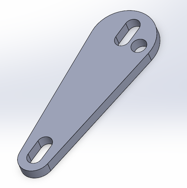
Figure 1. Support used for securing Line Sensors
Bump Sensors
We used bump sensors made for Romi, using both left and right modules. These bump sensors are used to detect collision, which will tell Romi the next steps. We attached these to the front of the Romi robot.
| Purpose | Pin Selection | Function |
|---|---|---|
| Bump 0 | PA12 | GPIO |
| Bump 1 | PA11 | GPIO |
| Bump 2 | PB12 | GPIO |
| Bump 3 | PB11 | GPIO |
| Bump 4 | PB15 | GPIO |
| Bump 5 | PB14 | GPIO |
| GND | GND | - |
| GND | GND | - |
Theory
Two forms of estimation were used in this lab. First was a simple state estimator that took inputs and applied dynamics equations and the RK4 solver to guess where ROMI would be the next time the task ran. It would continue to add to that value in hopes that it stayed accurate. The second was a discretized version of the system with a feedback loop. Using system dynamic equations and an observer gain matrix, new equations were used that directly computed the next state of ROMI given its current state. The equations and matrices used are as follows (exact numerical values not shown):
State Estimation:
x_dot = A x + B u (Eq. 1)
y = C x + D u (Eq. 2)
The A, B, C, and D matrices are based on ROMI dynamics, using the following state, input, and output definitions:
x = [Ω_l, Ω_r, s, φ]^T (Eq. 3)
u = [V_l, V_r]^T (Eq. 4)
y = [s_l, s_r, φ, φ_dot]^T (Eq. 5)
Discretized Estimation:
x_{k+1} = A_d x_k + B_d u* (Eq. 6)
y_k = C x_k (Eq. 7)
Where A_d and B_d are the discretized versions of A_o and B_o, defined as:
A_o = A − L C (Eq. 8)
B_o = B L (Eq. 9)
The observer input vector is:
u* = [V_l, V_r, s_l, s_r, φ, φ_dot]^T (Eq. 10)
The total distance travelled (s), is the only state there is no direct measurement for hence the use of an observer.
Test Results and Performance
Test Results
Velocity Plots testing
After pressing the go command “s”, we have the Romi go through 4 tests, each consisting of 10 step response tests. Those 4 tests are velocity for the left and right motor, and position for the left and right motor. These data points are automatically given to the user when running the PC script and plotted accordingly. The results are shown below in Figures 2-5.
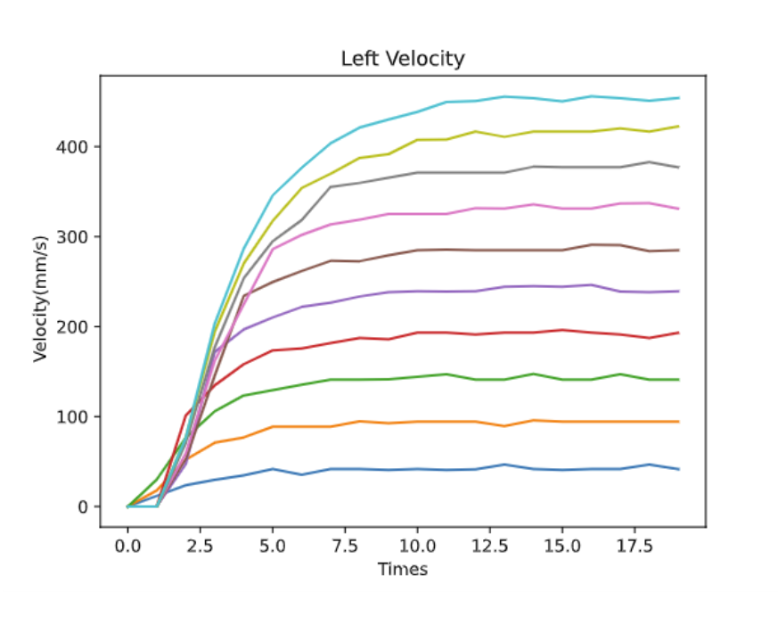
Figure 2. Left Motor Velocity Step Response
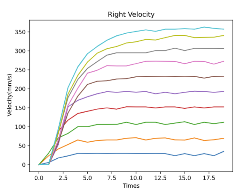
Figure 3. Right Motor Velocity Step Response
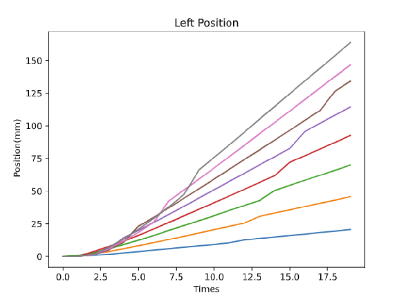
Figure 4. Left Motor Position Step Response
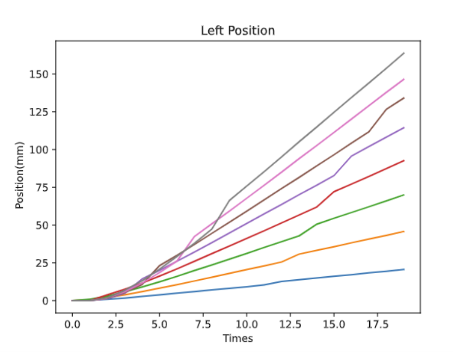
Figure 5. Right Motor Position Step Response
Based on these velocity graphs, it seems that our chosen frequencies were sufficient as it portrays a step response. Using the CSV files we obtained, we can then generate a time constant for both the left and right motors for the control theory task to be applied next week.
Closed Loop Control Testing
To tune Romi’s performance, we used our automatic data collection to run driving forward tests via our PC script. We started with only proportional control, running the motor at 200 mm/s, with K_P being the same for both motors, with Figure 6 being our first test. The next tests with Figures 7-8 are tests where we changed the Kp values, resulting in Figure 8, where we found a sufficient Kp value for this test period.
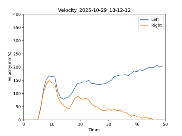
Figure 6. Velocity of both motors with Kpr = 0.25 and Kpl = 0.25
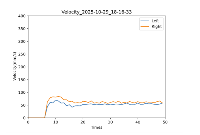
Figure 7. Velocity of both motors with Kpr = 0.1 and Kpl = 0.15
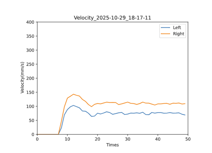
Figure 8. Velocity of both motors with Kpr = 0.1 and Kpl = 0.15 and Vref = 300 mm/s
After obtaining a relatively sufficient Kp, next we included integral control, controlling the Kp and Ki. Implementing both started of beneficial, as seen in Figure 9. We then raised Ki, in the next two Figures, 10 and 11, but it behaved erratically. Seeing as it was too much gain, we lowered Ki, but it still behaved erratically, so we were unsure where to continue from there.
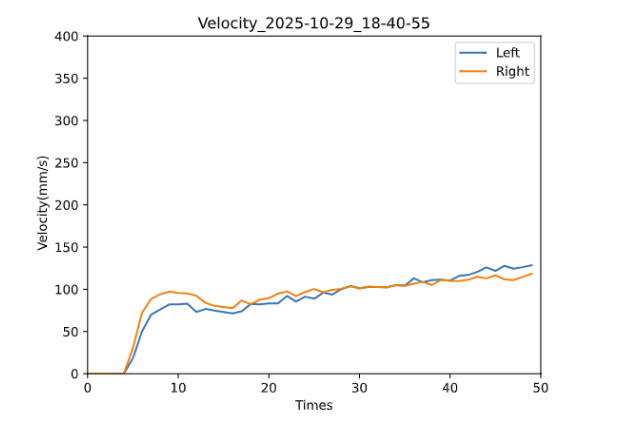
Figure 9. Velocity of both motors with Kpr = 0.1 and Kpl = 0.15, Kir = 0.5 and Kil = 0.5
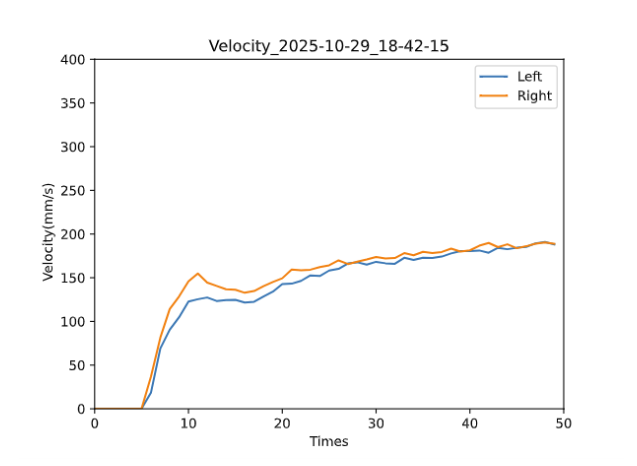
Figure 10. Velocity of both motors with Kpr = 0.1 and Kpl = 0.15, Kir = 2 and Kil = 2
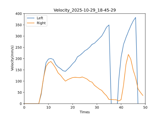
Figure 11. Velocity of both motors with Kpr = 0.1 and Kpl = 0.15, Kir = 2.5 and Kil = 2.5
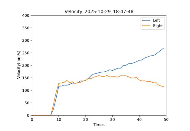
Figure 12. Velocity of both motors with Kpr = 0.1 and Kpl = 0.15, Kir = 2.1 and Kil = 2.1
Track Performance
Below are three videos containing our three attempts to autonomously drive the track. These attempts are rather inconsistant, which is due to our distance and yaw rates being thrown off while running the Romi.
Figure 13. Attempt #1
Figure 14. Attempt #2
Figure 15. Attempt #3
Task Diagrams
Below are the Finite State Machine transition diagrams for each task. They show the different states of the task, how they transition and what actions they take when transitioning.
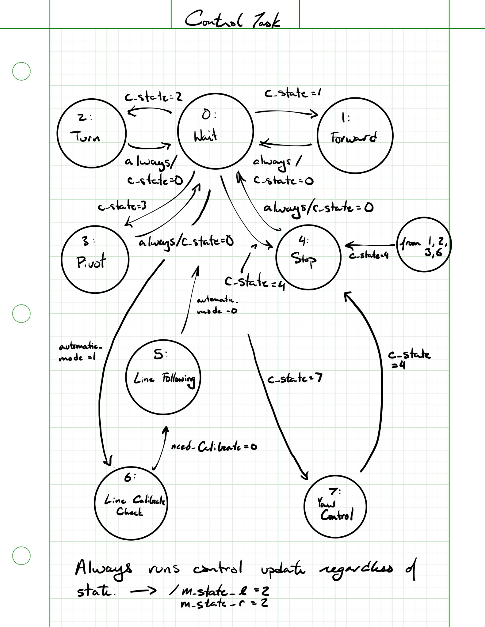
Figure 15. Control Task State Transition Diagram
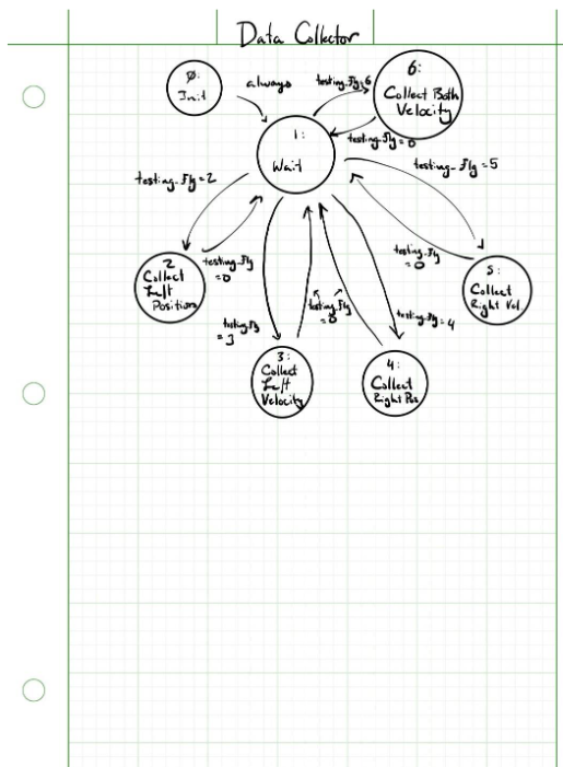
Figure 16. Data Collector Task State Transition Diagram
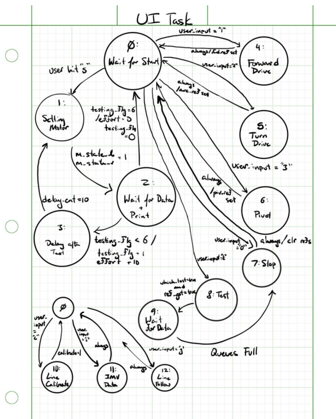
Figure 17. UI Task State Transition Diagram
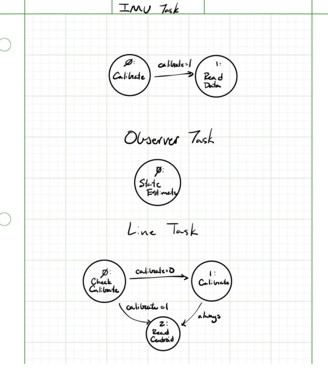
Figure 18. IMU Task State Transition Diagram
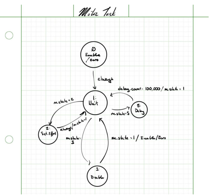
Figure 19. Motor Task State Transition Diagram
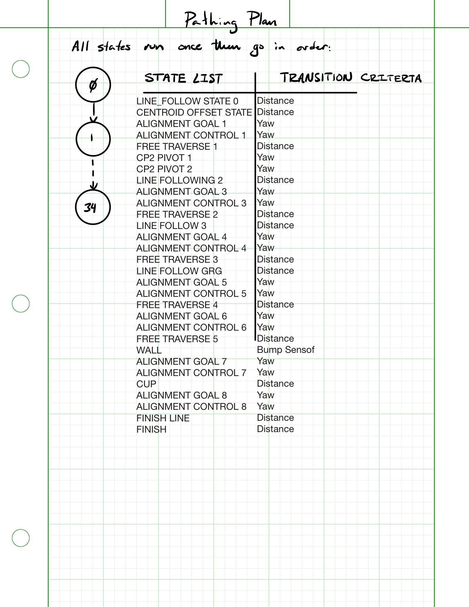
Figure 20. Pathing Plan Task State Transition Diagram
Priorities
Below is the priorities for our tasks.
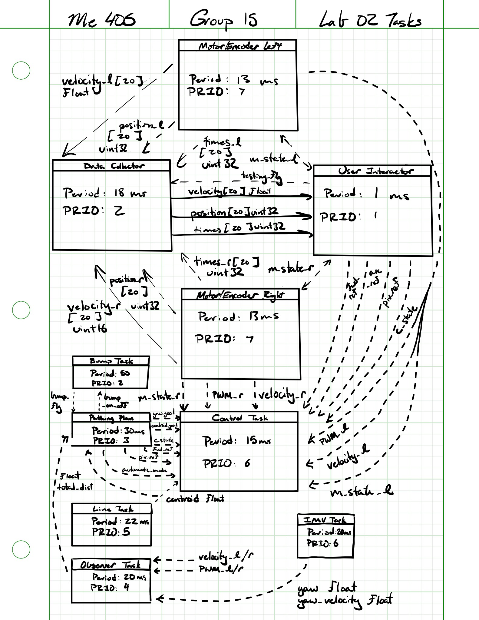
Figure 21. Control Task State Transition Diagram
Key takeaways
Our key takeaways from this project were learning how to successfully integrate all the hardware and bring the system close to achieving our goal. Moving forward, we would focus on improving our state estimation and refining the IMU outputs for distance and heading. These enhancements would increase consistency and would hopefully allow us to complete the course reliably.